2. Create MultiAssayExperiment Object
This section illustrates how to import data from multi-omics projects into the analysis process.
- If your dataset contains multiple omics data types, start from section 2.1
- If your dataset contains only a single omics data type, start from section 2.2
2.1 Multi-omics Data
When working with multiple omics datasets, users need to import and combine their data into a MultiAssayExperiment object. This process involves three main components: ① Sample phenotypic data; ② Omics data in SummarizedExperiment format; and ③ Sample relationship table. The following tutorial provides step-by-step examples for constructing each component. Example datasets are also provided for learning purposes.
Example dataset: 1. GitHub Download | 2. Baidu Netdisk Download
Navigation Guide
- ①Sample Phenotypic Data
- ②Reading Omics Data
- ③Creating Sample Relationship Table
- Integrating Components ①②③ to Construct MultiAssayExperiment Object
2.1.1 Sample phenotypic data
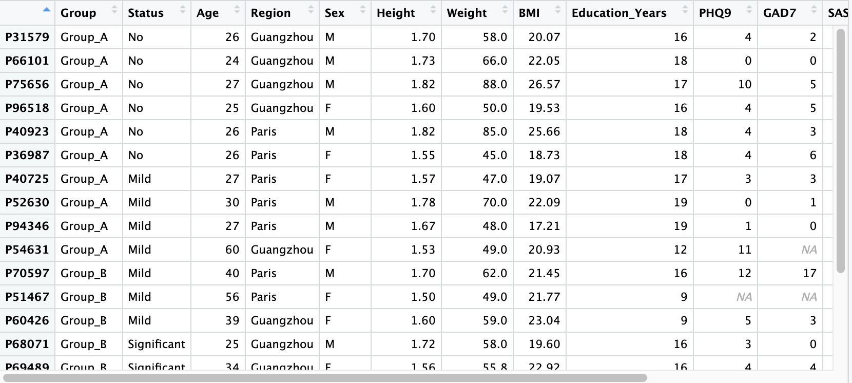
Sample-related data refers to the basic information of the subject, usually including: the subject's general demographic data (gender, age, residence, etc.), anthropometric data (height, weight, waist circumference, etc.), psychological scale score results (anxiety scale, depression scale, sleep scale, etc.), test results (blood routine, liver function, inflammatory factors, etc.).
① If there are missing values in the sample-related data, please leave them blank directly without using placeholders like NA, -, missing, etc.
② Please set the first column of the sample-related data as the Sample ID, and set it as the row names when reading (row.names = 1).
③ Sample ID must be unique and cannot be duplicated.
④ It is recommended to set the values of categorical variables in the data as strings rather than pure numbers to avoid unnecessary issues.
⑤ For the numbering scheme of project data before and after intervention for the same group of subjects, please refer to Chapter 10.3.
⑤ Special characters (-, ^) are not recommended in names. Please use underscores (_) for R compatibility.
## row.names=1
meta_data <- read.table('col.txt',header = T,row.names = 1)
2.1.2 Read microbiome data
Microbiome data refers to the result files containing the abundance information of microorganisms in each sample, which are generated by various upstream microbial annotation tools. Common result files include the following five types: ASV/OTU tables, abundance tables (kingdom, phylum, class, order, family, genus and species-level), generic-level abundance tables generated by MetaPhlan and Humann, Biom files, and QZV files specific to QIIME2. The module EMP_taxonomy_import supports the input of result files in all of the above formats and converts them into SummariseExperiment objects.
2.1.2.1 ASV/OTU forms
The # characters on the first and second lines of this file do not need to be modified. The data file must contains species annotation information.
① The data file must include a column named
taxonomy.② The
taxonomy column must contain microbial annotation.③ It is recommended to use
; character to separate microbial annotations.
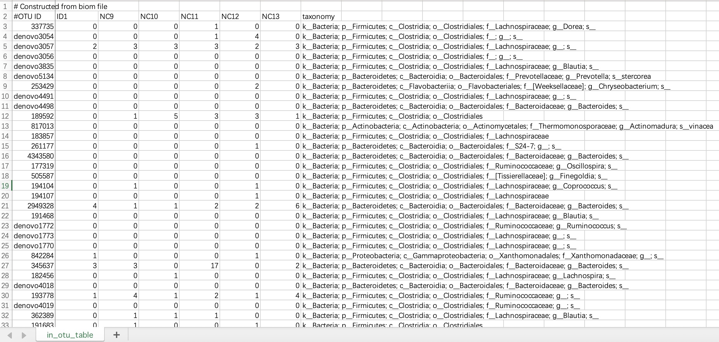
tax_data <- EMP_taxonomy_import('tax.txt',duplicate_feature=TRUE)
2.1.2.2 Abundance table (Kingdom, Phylum, family, genus, and species-level
Since high-taxonomic data can be converted to low-taxonomic data (e.g., Species data can be converted to Phylum data), it is recommended that users directly import data at the highest taxonomy level.
Module
EMP_taxonomy_import has a parameter assay_name which defaults to counts (absolute abundance). If the actual data is in relative abundance, you can input relative.
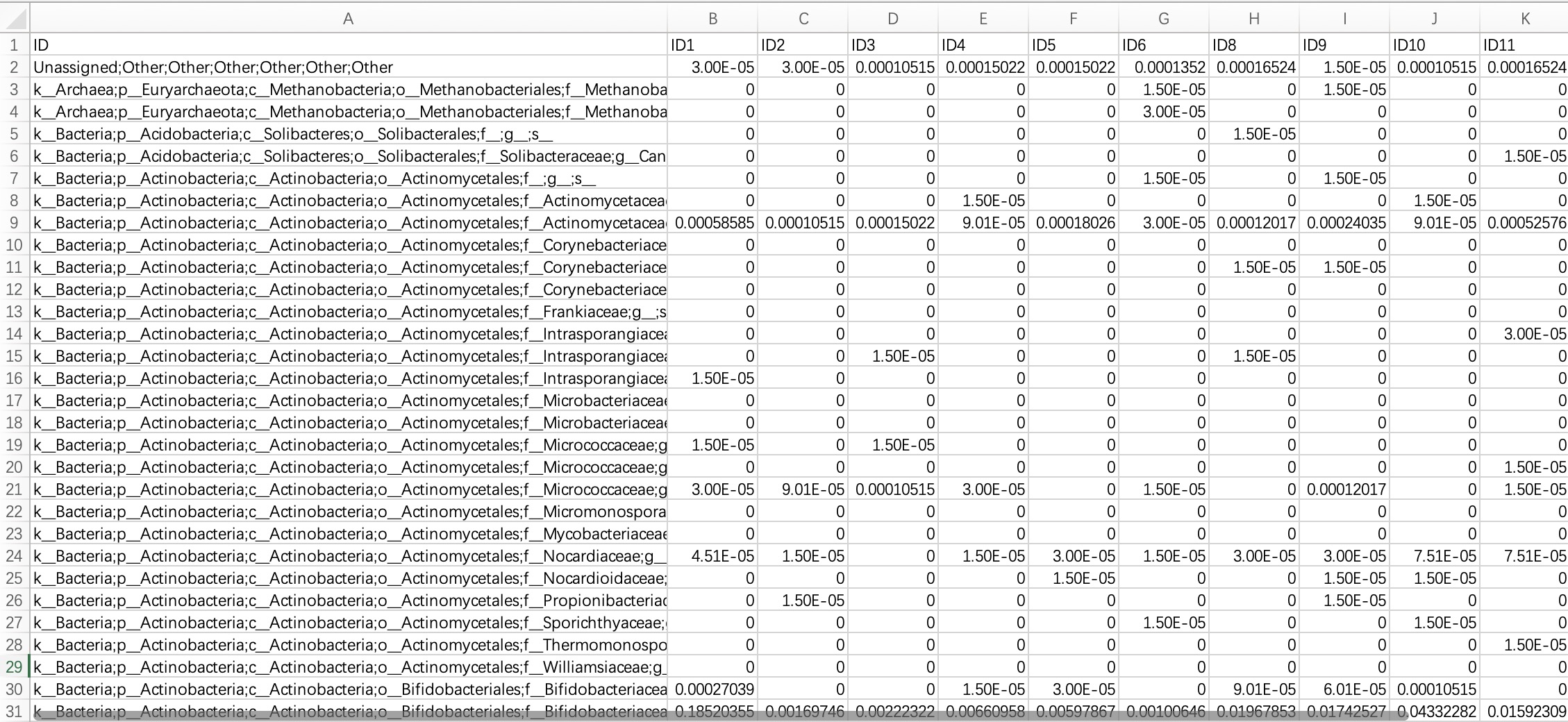
tax_data <- EMP_taxonomy_import('tax.txt')
2.1.2.3 Classification annotation table for MetaPhlan and Humann
The species annotations of this annotation table have a hierarchical structure and usually contain all the result information at each level of the genus and species of the phylum family. The module EMP_taxonomy_import can automatically identify annotation information at the highest classification level and import the complete classification data.
When the input data is in this format, users need to specify the parameter
humann_format=TRUE within the module EMP_taxonomy_import.

tax_data <- EMP_taxonomy_import('tax.txt',humann_format=TRUE)
2.1.2.4 Biom format files
The biom format is a common species annotation result file in the QIIME1 process, and some users will also save the species annotation file of the QIIME2 process in biom format for data storage. The module EMP_taxonomy_import can directly read the biom format file and import the data information.
When the input data is in this format, users need to specify the parameter
file_format='biom' within the module EMP_taxonomy_import.
tax_data <- EMP_taxonomy_import('tax.biom',
                                file_format='biom',duplicate_feature=TRUE)
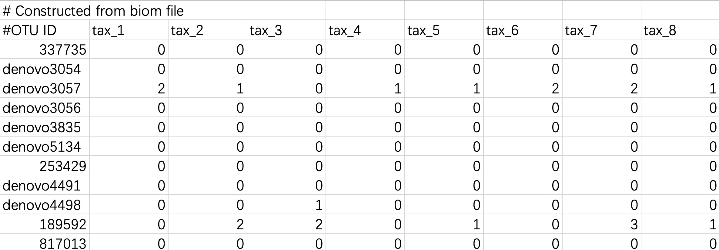
2.1.2.5 Tabular files converted from Biom format files
Biom files can be converted into tabular files using the Biom Convert method, or imported directly.
When the input data is in this format, users do not need to modify the header and # character.
tax_data <- EMP_taxonomy_import('tax.txt',duplicate_feature=TRUE)
2.1.2.6 QZV format file
In the Qiime2 process, the qiime taxa barplot generates a QZV file of microbial annotation results. The module EMP_taxonomy_import can directly read the QZV format file and import the data information.
When the input data is in this format, users need to specify the parameter
file_format='qzv' within the module EMP_taxonomy_import.
tax_data <- EMP_taxonomy_import('tax.qzv',
                                file_format='qzv',duplicate_feature=TRUE)
2.1.3 KO/EC omics data
KO/EC omics data are derived from functional annotations based on the KEGG database and primarily consist of two functional identifier systems: KO (KEGG Orthology) and EC (Enzyme Commission). These data are typically generated from metagenomic sequencing results analyzed by tools such as HUMAnN or PICRUSt2, and are used to characterize the potential metabolic functions and pathway activities of microbial communities. During import, the tool supports reading standard tabular files in which rows represent KO/EC functional features, columns represent samples, and cell values generally indicate the abundance or count of each function.
Primary Annotation Types:
- KO (KEGG Orthology): KEGG Orthology identifiers are used to associate gene functions with KEGG metabolic pathways.
- EC (Enzyme Commission): Enzyme Commission numbers provide a systematic classification and coding scheme for enzymes.
2.1.3.1 Standard tabular form
KO/EC omics project data in common format refers to metagenomic or metatranscriptomic annotated result files annotated with KO or EC ID. The module EMP_function_import can directly read the annotation table and query the corresponding annotation information integrated by the KEGG database.
① In the encoding, use only pure KO and EC ID, for example: instead of KO:K00010, use only K00010; instead of ec:1.1.1.1, use only 1.1.1.1.
② Within the module
EMP_function_import, the parameter assay_name defaults to counts (absolute abundance). Users should input TPM, FPKM, etc., based on the actual data.
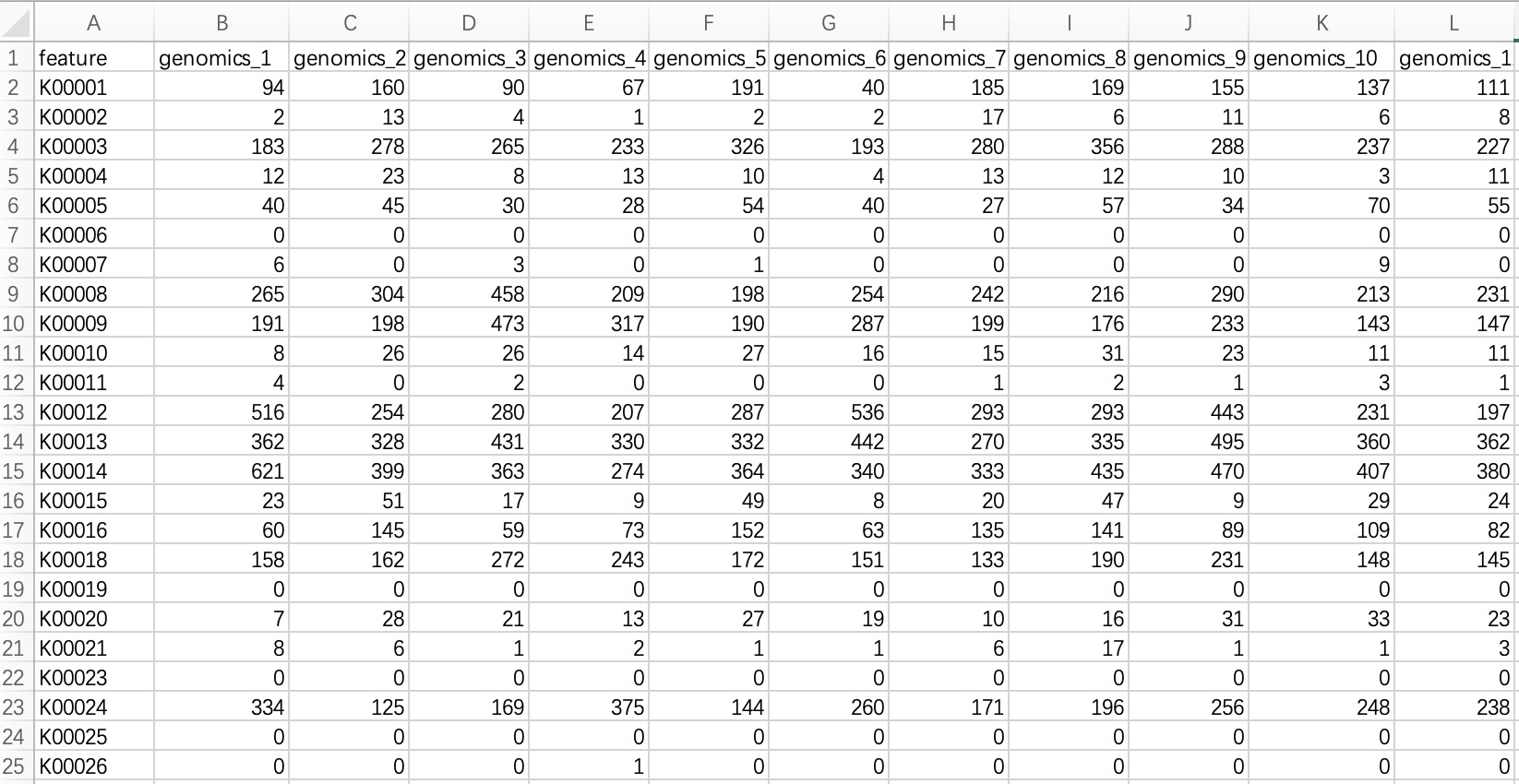
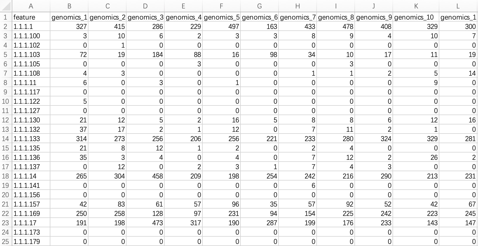
ko_data <- EMP_function_import('ko.txt',type = 'ko')
ec_data <- EMP_function_import('ec.txt',type = 'ec')
2.1.3.2 Humann format
KO/EC omics project data in Humann format refers to the hierarchical KO/EC annotation tables generated by the Humann tool. The module EMP_function_import ignores the information of UNGROUPED, directly reads the comment table, and queries the KEGG database to integrate the corresponding comment information.
The header of the file needs to be cleaned up and characters such as # removed.
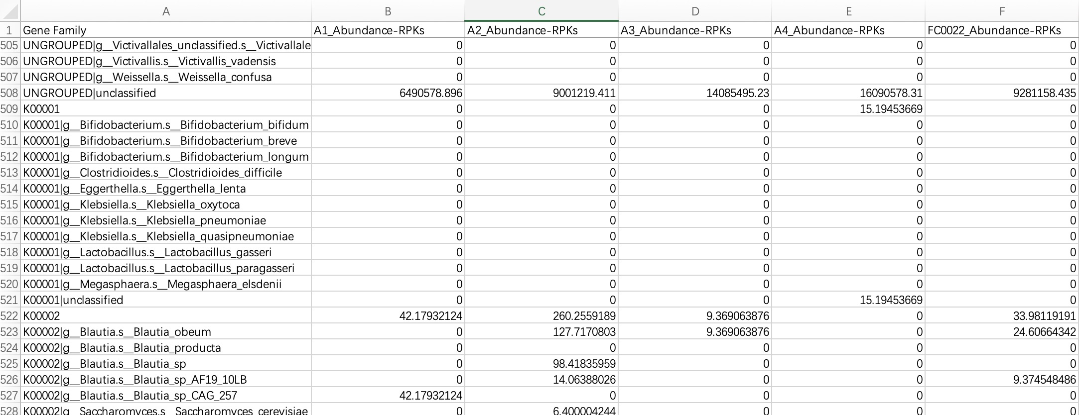
ko_data <- EMP_function_import('ko.txt',type = 'ko',humann_format = TRUE)
2.1.4 Standard table information
Standard tabular data usually refers to data such as transcriptome or metabolome, which has no special format and can be imported directly.
2.1.4.1 Table without feature annotation information
This data is commonly used in transcriptome or genomic data, with "rows" as features and "columns" as samples.
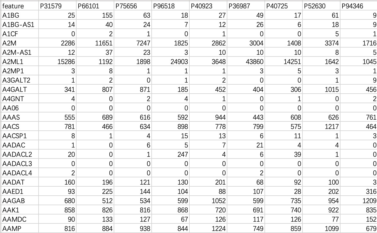
tran_data <- EMP_normal_import('tran.txt')
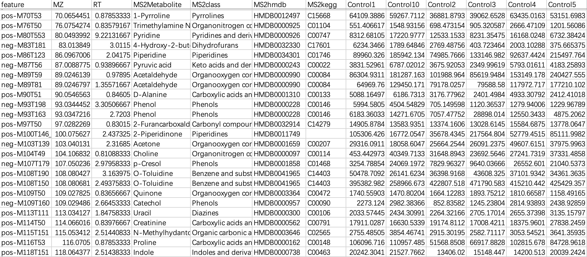
2.1.4.2 Table with feature annotation information
This data is commonly used in metabolomics data, with "rows" as features and "columns" as sampleID and feature-related annotations. When importing this kind of data, users need to specify a sampleID column.
① Users can directly specify the sampleID using parameter
sampleID.② Users can directly specify the sampleID using the relationship table.
# specify the sampleID using parameter sampleID
sample_ID <- c("Control1", "Control10", "Control2", "Control3", "Control4",
        "Control5", "Control6", "Control7", "Control8", "Control9",
        "Treat10", "Treat1", "Treat2", "Treat3", "Treat4", "Treat5",
        "Treat6", "Treat7", "Treat8", "Treat9")
metbol_data <- EMP_normal_import('metabol.txt',sampleID = sample_ID)

# specify the sampleID using the relationship table
metbol_data <- EMP_normal_import('metabol.txt',sampleID = sample_ID,
                                 dfmap = dfmap,assay = 'untarget_metabol')
2.1.5 Creating a Sample Mapping Table Linking Assay Samples to Subject IDs
After importing the data, two key components have been loaded: ① Omics data stored in SummarizedExperiment format, and ② Sample phenotypic data. The next step is to construct the ③ Sample mapping table.
The primary purpose of this table is to resolve the common issue of inconsistent sample naming across multiple omics datasets. In many studies, different omics platforms or experimental batches may assign different sample identifiers to the same subject, preventing direct matching between expression matrices and phenotypic data. The sample mapping table is designed to establish a clear correspondence between them.
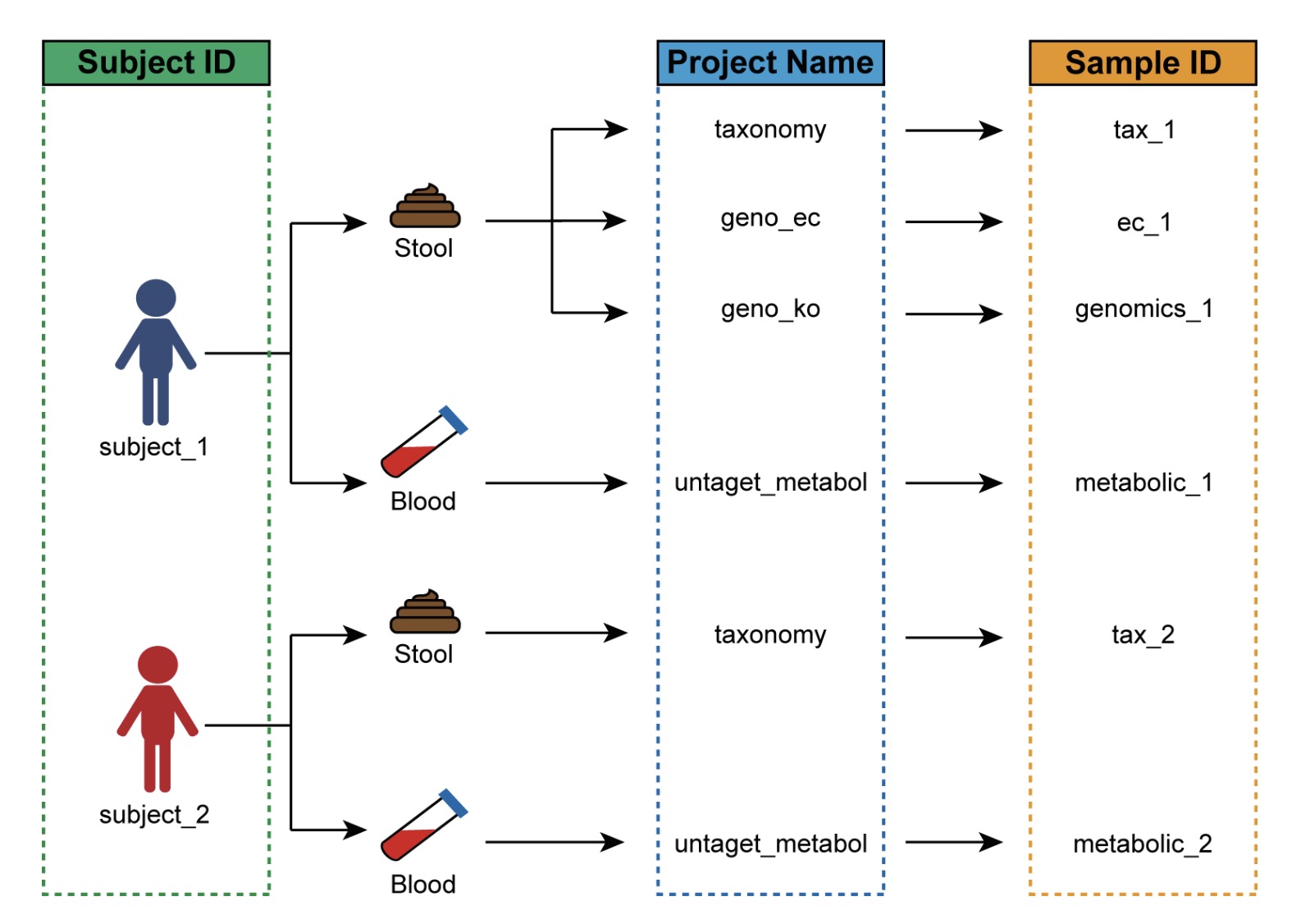
For example, in a human study involving multiple omics assays:
Each subject has a unique identifier (e.g., P1, P2, P3…);
The same subject may provide multiple biological samples for different omics assays, such as:
○ 16S rRNA taxonomic annotation (taxonomy), with sample IDs such as tax_1, tax_2, tax_3,…;
○ Microbial functional gene KO annotation (geno_ko), with sample IDs such as genomics_1, genomics_2, genomics_3,…
In this case, the sample mapping table must link the subject ID P1 in the phenotypic data to the corresponding assay-specific sample IDs—tax_1 and genomics_1.
Once this table is established, users can seamlessly integrate all data into a MultiAssayExperiment object. In subsequent analyses, the EasyMultiProfiler package will automatically use this mapping to replace all assay-specific sample IDs with the unified subject identifiers, ensuring data consistency and analytical reproducibility.
A mapping-based workflow offers the following advantages:
Data Integration and Consistency: Ensures accurate alignment and merging of sample information across different omics datasets.
Automated Processing: Enables fully automated data handling without manual renaming, eliminating inconsistencies caused by naming variations.
Streamlined Analysis: Simplifies the analytical workflow by automatically harmonizing sample identifiers, reducing manual errors, and processing time.
If the sample names in the omics expression matrix already match those in the phenotypic data, you can simply create a mapping table using identical names.
🏷 Example: Creating a mapping table linking subject IDs and assay-specific sample identifiers.
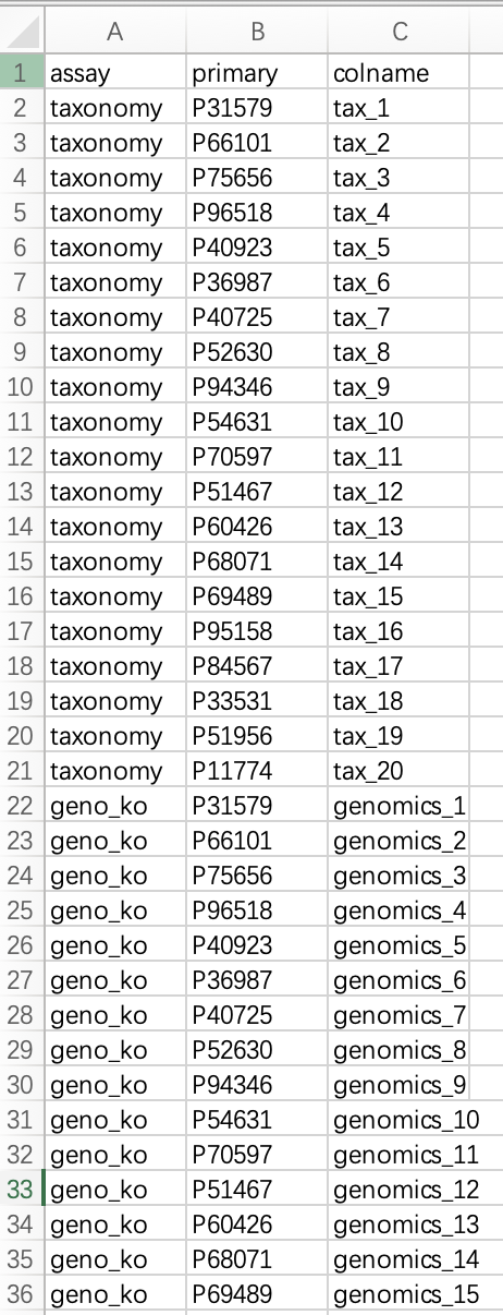
① The mapping table must contain the following three columns:
assay (name of the omics assay), primary (subject identifier), and colname (sample identifier in the omics assay).②
assay refers to the user-defined name of the omics dataset. primary corresponds to the sample name in the phenotypic data. colname is the sample name as it appears in the expression matrix of the corresponding assay.③ Each sample identifier in an omics assay must have a one-to-one match in the
colname column of the mapping table.④ For naming schemes in longitudinal or pre-/post-intervention studies, please refer to Section 10.3.
This table must be saved as a file and read into R. Alternatively, users can create the data frame directly in R.
dfmap <- read.table('dfmap.txt',header=TRUE,sep='\t')
2.1.6 Integrate all data into the MultiAssayExperiment object
① In this example,
dfmap refers to the relationship table in section 2.1.5.② The
assay column in the relationship table must be converted to a factor.③ Names in
objlist must match the project names in the assay column of the relationship table.④ If assembly fails, users can check the data using the module
MultiAssayExperiment::prepMultiAssay(objlist, meta_data, dfmap).⑤ For more detailed information about the
MultiAssayExperiment package, refe to this tutorial.
#### The assay column in the relationship table must be converted to a factor
dfmap$assay <- as.factor(dfmap$assay)

#### Names in objlist must match the project names in the assay column of the relationship table
objlist <- list("taxonomy" = tax_data,
                "geno_ko" = ko_data,
                "geno_ec" = ec_data,
                "untarget_metabol" = metbol_data,
                "host_gene" = geno_data)

MAE <- MultiAssayExperiment::MultiAssayExperiment(experiments=objlist,
                                                  colData=meta_data,
                                                  sampleMap=dfmap)
2.2 Quickly create a MultiAssayExperiment object for a single-omic project
When the users only have a single-omic project data (for example, microbiome project data or transcriptomics project data), the module EMP_easy_import can be used to quickly build a MAE object and directly perform downstream analysis processes.
① The parameter
type includes four options: tax, ko, ec, and normal. Users should determine which to use based on the context.② For single-omic project where no relationship table is involved, the sampleID in the abundance matrix must match those in the Sample phenotypic data.
10.6 Microbiome Analysis
10.7 Transcriptomics Analysis
10.8 Metabolomics Analysis
2.3 MultiAssayExperiment object storage and reading
Once the MAE object has been created, it can be stored locally for direct reading during the next analysis without having to repeat the creation step.
Before storing, make sure to set R's local working directory correctly, and the data files will be stored in this working directory.
# Save in your working diectory
saveRDS(MAE,file = 'MAE.rds')
# Load the object
MAE <- readRDS(file = 'MAE.rds')
2.4 Demo data and script for build MAE obejct
Demo data:Click this
library(EasyMultiProfiler)

## Load meta data
meta_data <- read.table('coldata.txt',header = T,row.names = 1)

## Load dfmap
dfmap <-read.table('dfmap.txt',header = T) %>%
  dplyr::mutate(assay = factor(assay))

## Load omics data
tax_data <- EMP_taxonomy_import('tax.txt')

ko_data <- EMP_function_import('ko.txt',type = 'ko')

ec_data <- EMP_function_import('ec.txt',type = 'ec')

metbol_data <- EMP_normal_import('metabol.txt',dfmap = dfmap,assay  = 'untarget_metabol')

geno_data <- EMP_normal_import('tran.txt',dfmap = dfmap,assay  = 'host_gene')

## Combine into list
objlist <- list("taxonomy" = tax_data,
                "geno_ko" = ko_data,
                "geno_ec" = ec_data,
                "untarget_metabol" = metbol_data,
                "host_gene" = geno_data
)

## Create MAE object
MAE <- MultiAssayExperiment::MultiAssayExperiment(objlist, meta_data, dfmap)

## Save to file for future use without re-assembly
saveRDS(object = MAE,file = 'demo_data.rds')

## Load the saved data directly next time
MAE <- readRDS('demo_data.rds')